A relatively simple function for generating presentation-ready phylogenies, given a set of common or scientific names. It works best for a few species, since the goal is to make a phylogeny for pedagogical purposes, so the focus is on details, not quantity.
showPhylo(
  speciesNames,
  nameType,
  dateTree = TRUE,
  labelType = "b",
  labelOffset = 0.45,
  aspectRatio = 1,
  pic = "wiki",
  dotsConnectText = FALSE,
  picSize = 1,
  picSaveDir,
  optPicWidth = 200,
  picBorderWidth = 10,
  picBorderCol = "#363636",
  openDir = FALSE,
  xAxisPad = 0.2,
  xTitlePad = 20,
  numXlabs = 8,
  textScalar = 1,
  xTitleScalar = 1,
  phyloThickness = 1.2,
  phyloCol = "#363636",
  textCol = "#363636",
  plotMar = c(t = 0.02, r = 0.5, b = 0.02, l = 0.02),
  clearCache = FALSE,
  quiet = TRUE,
  silent = FALSE,
  ...
)
Arguments
| speciesNames | a name or vector of common or scientific names of organisms of interest (in quotes) |
|---|---|
| nameType | what type of name are you supplying? Either "sci" or "common" |
| dateTree | try to scale the tree to estimated divergence times? Uses |
| labelType | which names to label tree "leaves"? Options= "s" for scientific, "c" for common, and "b" for both (default="b") |
| labelOffset | how far from the tree tips do you want to put labels? default=0.3 (in proportion of x-axis units) |
| aspectRatio | doesn't actually work yet; the output phylogeny is always square for the moment |
| pic | what type of species image do you want to plot? options="wiki" (Wikipedia page profile image), "phylopic" (species' silhouette from the PhyloPic repository), "cust" (custom images: must be named .jpg or .png with names matching speciesNames in the picSaveDir folder), or "none" |
| dotsConnectText | do you want a dotted line to go from the text to the labels? default=FALSE |
| picSize | how big to scale images, where 1=100%; .5=50%; default=1 |
| picSaveDir | location for saving downloaded images; default=fs::path(tempdir(),"showPhylo") |
| optPicWidth | picture width in pixels for optimized versions of images saved if using pic="cust"; default= 200 |
| picBorderWidth | for pic="wiki" or "cust," what size border would you like around your image (as a %); default=10 |
| picBorderCol | color of image border; default="# 363636" (a dark, near-black color) |
| openDir | for pic="wiki" or "cust," do you want to open the picSaveDir after processing files? default=FALSE |
| xAxisPad | spacing between the phylogeny and the x-axis (scale is 1 is the distance between two sister taxa); default=.2 |
| xTitlePad | spacing between x-axis title and x numbers; default=20 |
| numXlabs | the number of year markers on the x-axis; default=8 |
| textScalar | multiplier of text size for labels and axis numbers; default=1 |
| xTitleScalar | multiplier of x-axis title size; default=1 |
| phyloThickness | how thick to make the phylogeny lines; default=1.2 |
| phyloCol | color of the phylogeny lines; default= "# 363636" |
| textCol | color of the axis and tip labels; default= "# 363636" |
| plotMar | margins around the plot area in proportional screen width units; note the right margin is much wider to make room for tip labels; default=c(t=.02,r=.4,b=.02,l=.02) for top, right, bottom, left |
| clearCache | delete cached images and taxonomic names? Passed to getPhyloNames, getWikiPics, and also applies to optimized custom images; default=FALSE |
| quiet | suppress verbose feedback from the taxize package? Passed to getPhyloNames and get WikiPic helper functions. Default=TRUE |
| silent | suppress all console output? (Mainly for R documentation); Default=FALSE |
| ... | pass other parameters to |
| datelifePartialMatch | use use source trees even if they only match some of the desired taxa; affects the |
Details
You have the ability to look up matching common or scientific names for taxa, plot them in an evolutionary tree based on the Open Tree of Life Project, date taxa using datelife_search, if data are available, plot a phylopic (i.e. a silhouette of the organism) if available, pull down the profile image from each organism's Wikipedia page, or provide a custom image, and label the pictures with the scientific and common names. The result is a customizable ggplot2 object. This is a convenience wrapper that merges functionality from ggplot2, ggtree, datelife, rotl,and taxize, among other packages.
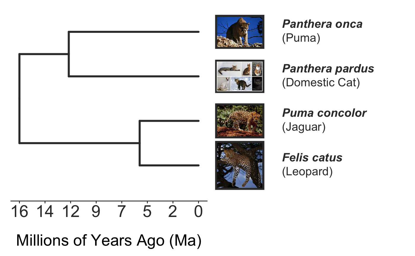
The impetus for this package was the need to make a figure showing that the many animals we call "panthers" are actually really distantly related cat species. Our genetic rescue lesson, sponsored by Dr. Sarah Fitzpatrick's lab, uses the example of the Florida panther as a charismatic application of her research (which mostly uses guppies as a model for understanding how gene flow can save small, highly inbred populations from extinction).
Examples
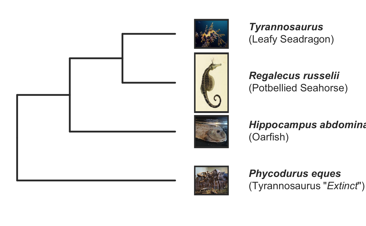
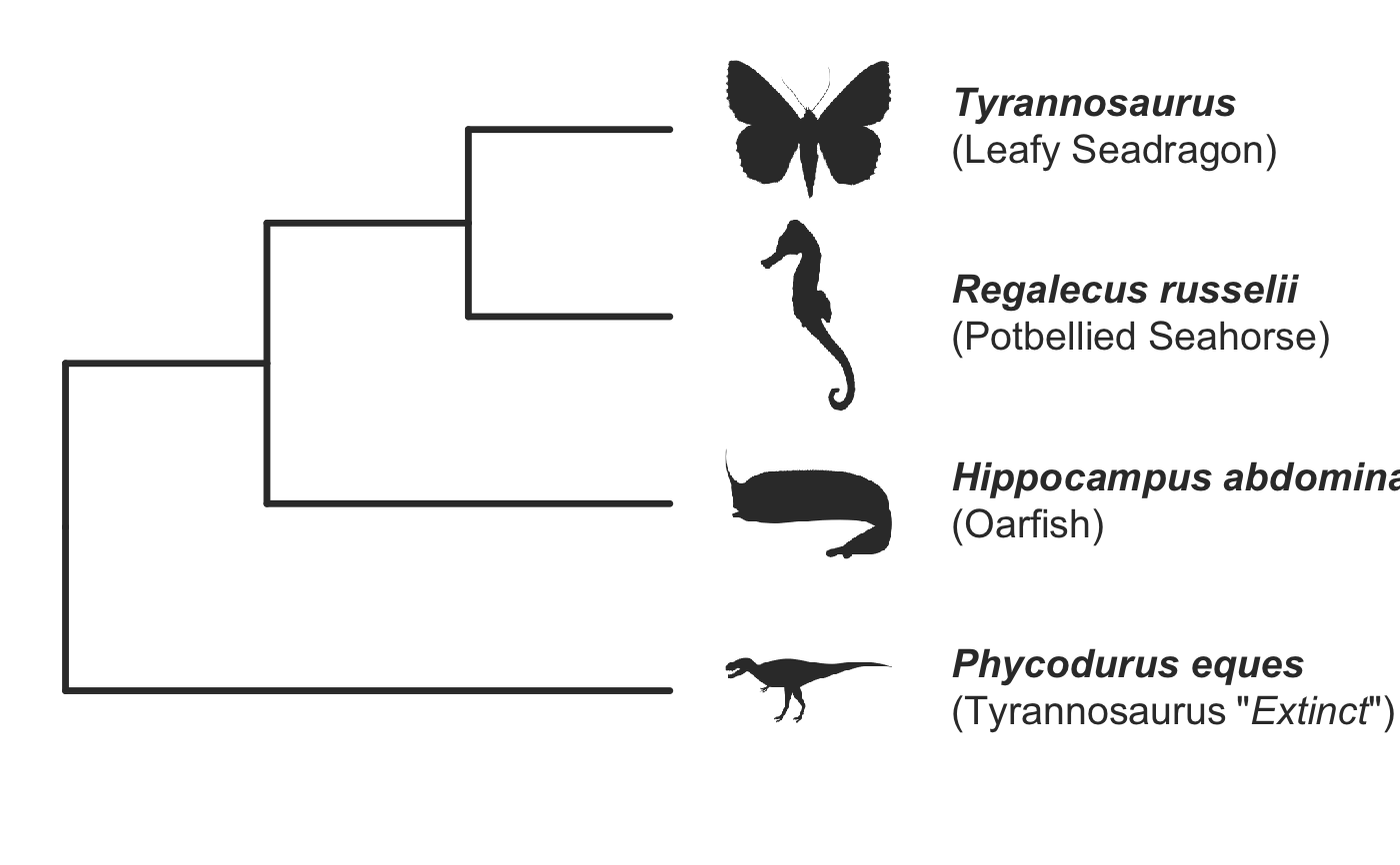
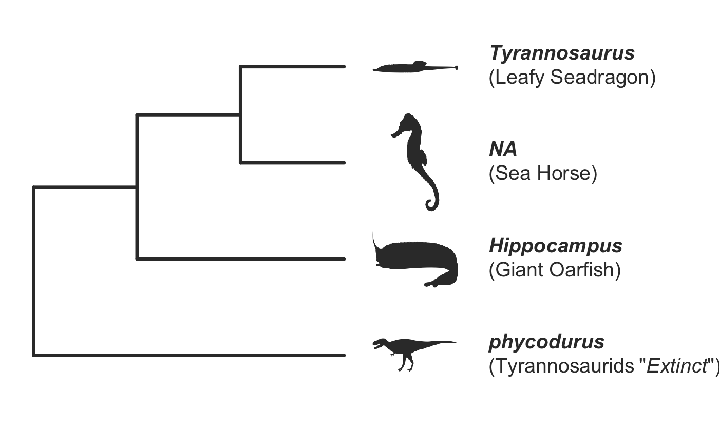
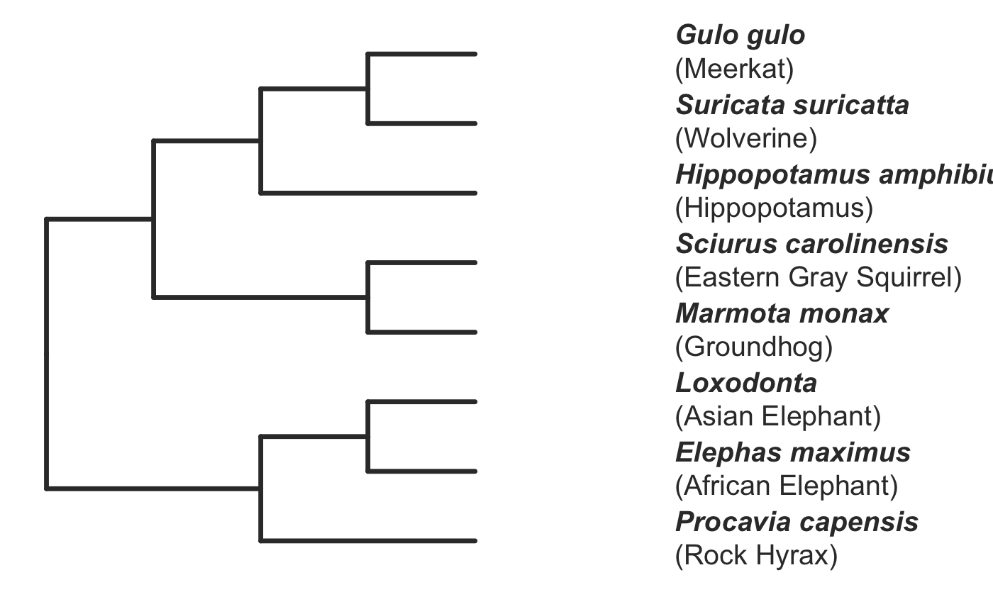
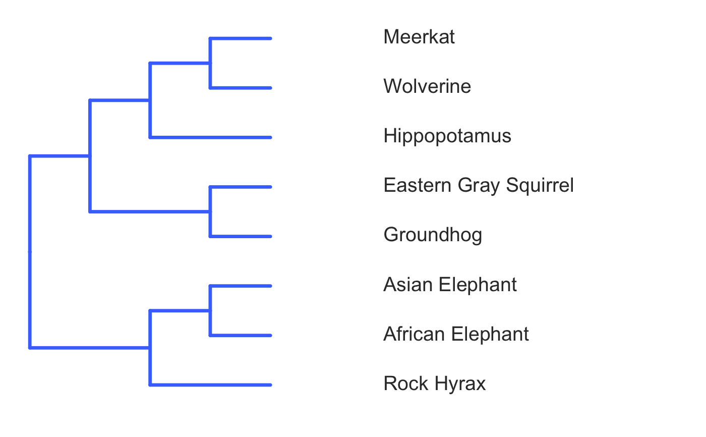
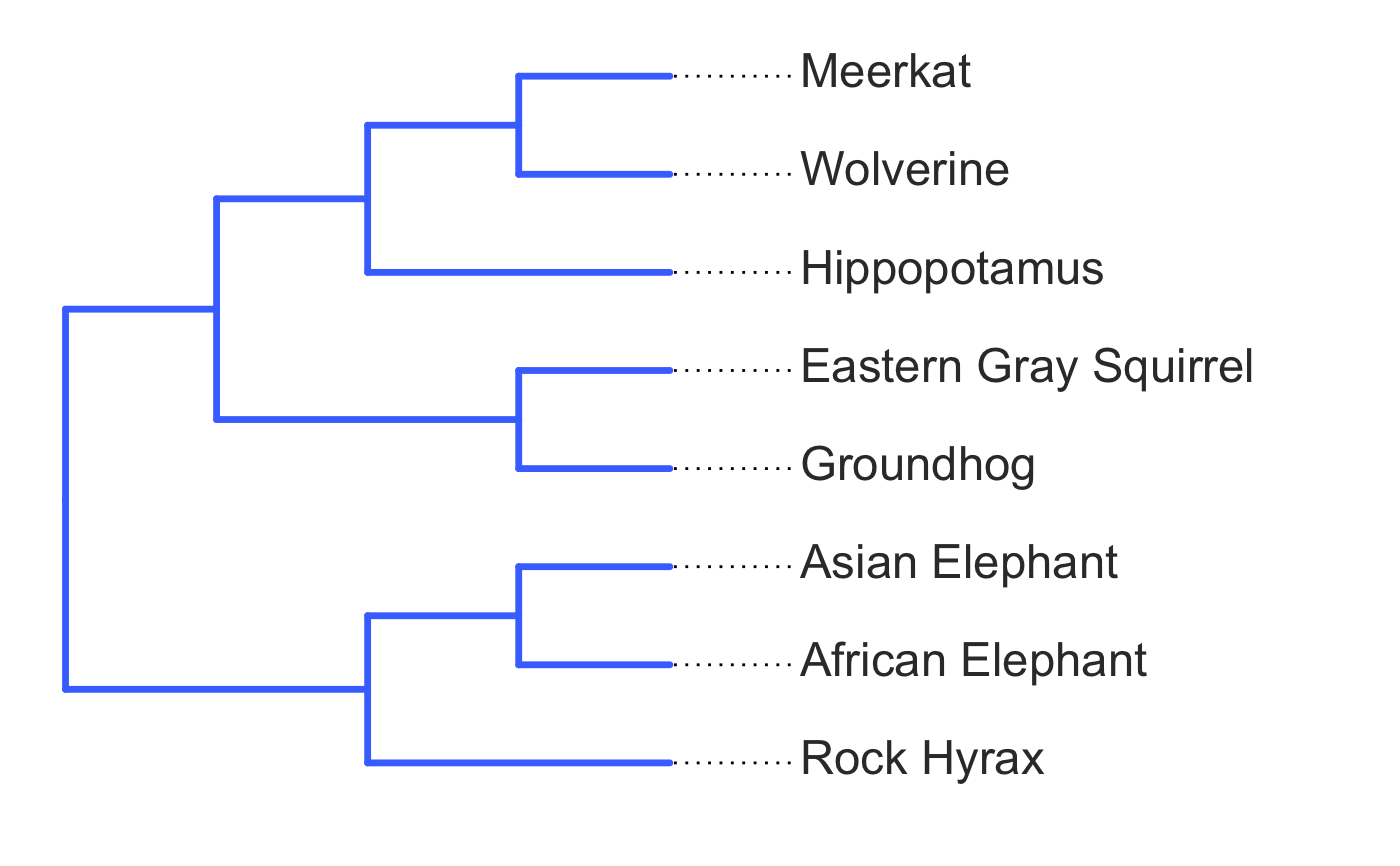
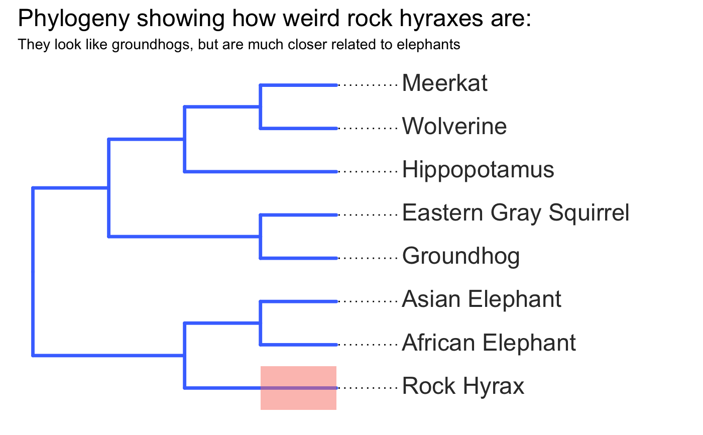
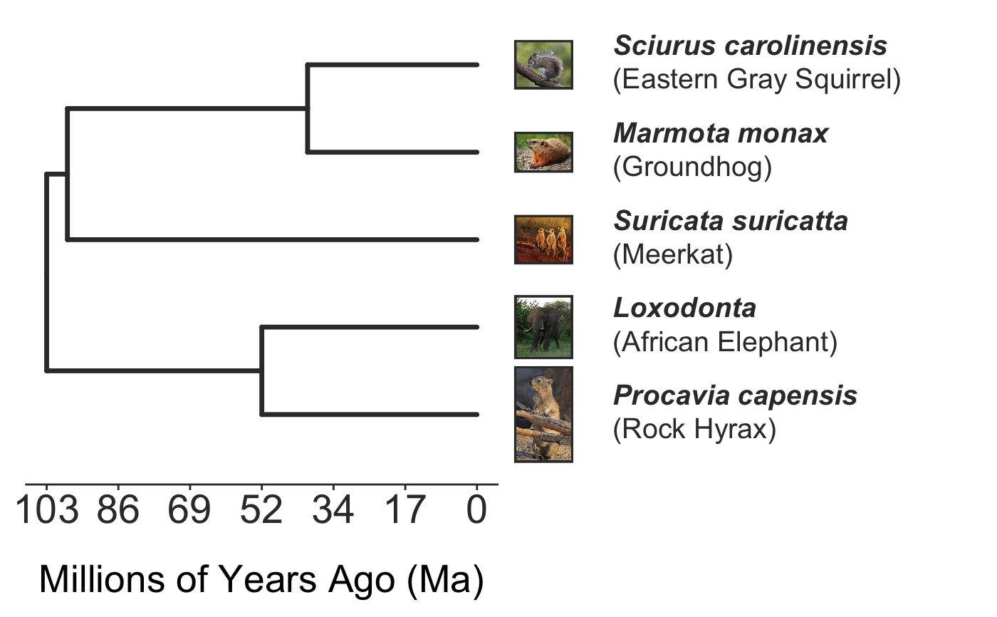
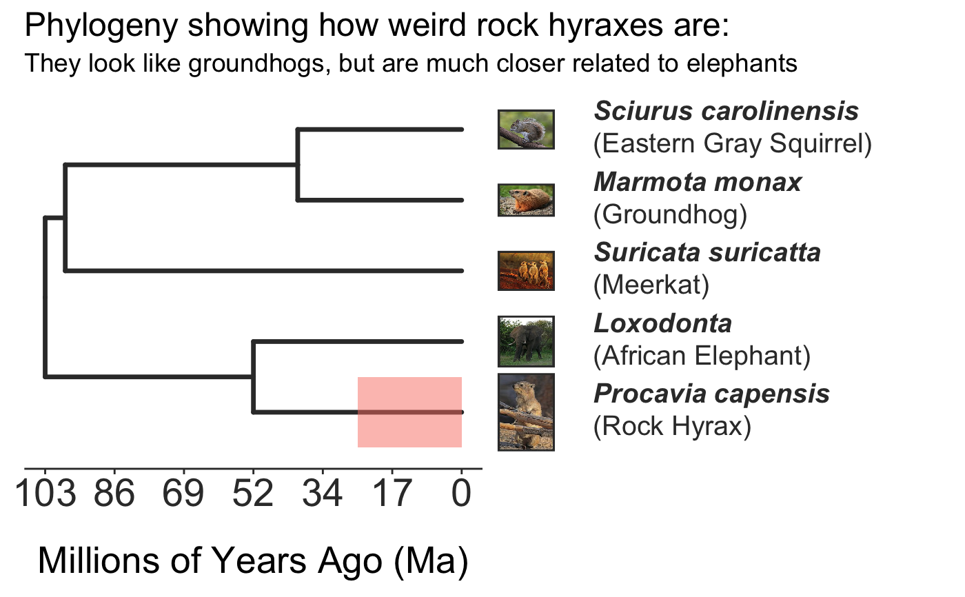
invisible({require(ggplot2);require(ggtree)}) # declare some species common names speciesNames <- c("puma","leopard","jaguar","domestic cat") # Make a dated phylogeny with them (by default, median divergence times are estimated # using the datelife package and images are added from Wikipedia) # *Note* I'm using silent=TRUE to suppress all output to the console for this document; # You will usually want to leave silent=FALSE (default) to see what's happening # and diagnose problems. There are a lot of steps happening behind the scenes showPhylo(speciesNames,"c",silent=TRUE)# If a particular combination of organisms lacks divergence time data # (especially extinct species), causing an error (e.g. this) if (FALSE) { showPhylo(c("potbellied seahorse","leafy seadragon", "oarfish","Tyrannosaurus"),"common",silent=TRUE) } # you can possibly still produce an undated phylogeny (cladogram) using the open # tree of life data; also modified plot margin to have more space for taxa labels showPhylo(c("potbellied seahorse","leafy seadragon", "oarfish","Tyrannosaurus"),"c",dateTree=FALSE,picSize=.8,silent=TRUE)#> Warning: Double check output. You've got some matching scientific and common names. Did you supply the correct nameType?# Instead of Wikipedia images for each species, we can try to find a phylopic (silhouette) showPhylo(c("potbellied seahorse","leafy seadragon","oarfish", "Tyrannosaurus"),"c",dateTree=FALSE,pic="phylopic",silent=TRUE)#> Warning: Double check output. You've got some matching scientific and common names. Did you supply the correct nameType?# In the case above, the butterfly was the wrong image, so we could try searching using the genus, # (note: change nameType to "scientific"); showPhylo(c("Hippocampus","phycodurus","Regalecus","Tyrannosaurus"), "scientific",dateTree=FALSE,pic="p",silent=TRUE)# Not great, but phylopic is open source, # so you can upload your own silhouettes # If you have a ton of species, you can just say no pics speciesNames<-c("rock hyrax","Hippopotamus","Eastern gray squirrel","Asian elephant", "African elephant","groundhog","meerkat","wolverine") showPhylo(speciesNames,"c",pic="n",dateTree=FALSE,silent=TRUE)# Doesn't look great, so we can connect the tree tips with the text # and make the tree blue (why not?); Also, let's just show common names, # and add more space in the right margin for all the text showPhylo(speciesNames,"c",pic="n",dateTree=FALSE,phyloCol="royalblue1", labelType="c",plotMar=c(r=".6"),silent=TRUE)# We could also shorten the gap between the tree and the text, add connecting dots, # and increase text size g<-showPhylo(speciesNames,"c",pic="n",dateTree=FALSE,phyloCol="royalblue1",dotsConnectText=TRUE, labelType="c",labelOffset=.2,textScalar=1.2 ,silent=TRUE)# once we're satisfied with the tree, we can edit it like any other ggplot g2<-g+labs(title="Phylogeny showing how weird rock hyraxes are:", subtitle="They look like groundhogs, but are much closer related to elephants")+ theme(plot.title=element_text(size=18) ) # we can also use ggtree functions to do all sorts of stuff like highlight our key species # (you can figure out which node that is here with g2$data) g2+geom_highlight(mapping=aes(subset=node==6),fill="salmon")# OK, let's simplify it, add divergence time and get some pics back; also reduce pic size # and space between pic and text and only print 7 breaks in the x-scale speciesNames <- speciesNames[c(1,3,5,6,7)] g3<-showPhylo(speciesNames, "c" ,silent=TRUE,picSize=.5,labelOffset=0.3, numXlabs=7)# Last tweaks: let's highlight the hyrax branch and add our titles g3+geom_highlight(mapping=aes(subset=node==4),fill="salmon")+ labs(title="Phylogeny showing how weird rock hyraxes are:", subtitle="They look like groundhogs, but are much closer related to elephants")+ theme(plot.title=element_text(size=18),plot.subtitle=element_text(size=14))# to get the right output dimensions, you may need to play around with setting height & width # e.g. ggsave("hyrax.jpeg",height=3,width=3)